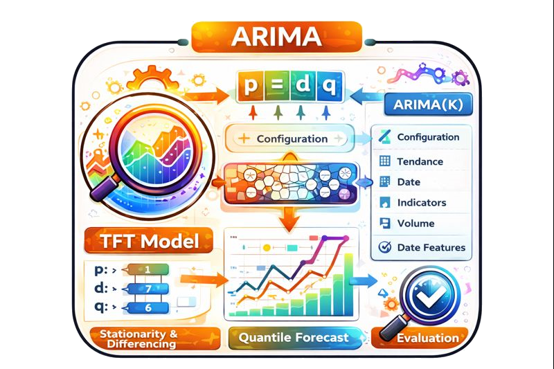
ARIMA Forecasting Core
ARIMA is the classic workhorse of time series forecasting. It decomposes a sequence into autoregressive memory, integration for trend stabilization, and a moving average noise filter. This gives a compact, interpretable baseline that stays stable under noisy crypto regimes.


How ARIMA Works
ARIMA models the conditional mean of a series after removing non-stationary drift. The autoregressive terms explain persistence, the integration operator stabilizes the mean, and the moving average terms compress correlated noise. This structure is stable, fast, and ideal for validating more complex models.
In crypto, ARIMA is used to detect short range momentum and reversal behavior, calibrate volatility baselines, and provide a transparent reference prediction that can be compared against transformer based forecasts.
- Stationarity testing via ADF and KPSS style checks.
- Order selection from ACF, PACF, and information criteria.
- Residual diagnostics to confirm white noise errors.
- Rolling refits to adapt to regime change without overfitting.
Normalize and Difference
Transform raw prices into returns, stabilize variance, then apply differencing to remove drift.
Select Orders
Search p, d, q using AIC and BIC while respecting short horizon market structure.
Fit and Validate
Estimate parameters, then verify residuals for independence and stable variance.
Forecast with Bands
Produce point forecasts with confidence intervals that feed the ensemble risk layer.
Core Equations
These equations describe the linear dynamics and the noise model. The parameters are optimized on rolling windows to remain stable in non-stationary markets.
Where ARIMA Fits
- Interpretable parameters that explain persistence and shock decay.
- Fast training for frequent recalibration across many assets.
- Reliable baseline for ensemble blending and anomaly detection.
- Linear structure struggles with abrupt regime shifts.
- No direct handling of exogenous signals without extension.
- Long horizon accuracy degrades in high volatility windows.
ARIMA serves as the statistical anchor in our prediction stack, especially for short horizon sanity checks and variance estimation.


